Introduction
Liquidity pools are a basic primitive of DeFi protocols and their respective tokens. Choosing to bootstrap initial liquidity via automated market makers rather than going through exchanges democratizes access to initial liquidity and saves money. Additionally it creates the opportunity to offer liquidity mining rewards (to varying degrees of effectiveness) to participants in order to incentivize locking liquidity in pools and incurring risk of impermanent loss. Liquidity bootstrapping strategies are generally not forward-looking; as rewards dry up liquidity progressively leaves the pool(s), hurting the long-term stability and viability. The problem is that reward schemes are currently based on the assumption that liquidity will grow indefinitely, an assumption that is fundamentally impossible in practice. One approach to combat this is protocol-owned liquidity, a system by which a DAO can take control of its own token liquidity by offering bonding discounts in exchange for participants locking up other tokens. In this piece I propose an alternative strategy - modeling a liquidity pool as a ‘quantum particle in a box’, in order to leverage the quantum wave function and the principle of quantum tunneling in order to produce rewards emissions that restrict liquidity to a particular range.
Background
‘Particle in a box’ is one of the generalized setups used to understand the behavior of fundamental particles as they interact with potential energy barriers. In the quantum mechanical world, particles are in fact wave functions, defined as Ψ(x). Schrodinger’s equation can then be used to understand the wave nature of the particle and is defined as:
H(t)|Ψ(t)> = iℏ d/dt|Ψ(t)> and H(x)Ψ(x) = E(x)Ψ(x)
(eq. 1.1)
Where H is the Hamiltonian operator, which is related to the kinetic and potential energy of the particle. This equation is solved to find particular functions Ψ(t) and Ψ(x) for different situations. These solutions can be exponential, sine-like, or take other forms. The setup to be applied to liquidity pools is that of a particle, modeled by the above function, between two potential barriers of height V_o where V_o > V_Ψ.
Transforming Coordinates
Typically these problems can be plotted on a graph where the x-axis represents space and the y-axis represents potential energy, measured in Joules. An allegory to these coordinates is needed to properly apply this concept to the world of token liquidity. There is also the question of how to represent mass within this system. For the moment I choose to ignore mass by setting all constants and mass within the Hamiltonian to be equal to one. Normally the hamiltonian would be written as: -(ℏ^2/2m)∇^2 + V but becomes -∇^2 +V where ∇^2 is the laplacian operator, or the second derivative of all spacial coordinates. For the x-axis coordinates, I choose total aggregate liquidity within the pool, valued in either ETH or USD, to be the units of the axis. For the y-axis, which normally would be defined as potential energy, I correlate this to the number of staking wallets in the pool. I chose this approach for two reasons: 1), the height of the potential well that is created by the two barriers in this setup is only important to model how emissions are generated, and 2), if the number of holders outside the pool is infinity, then the emissions can set to go to zero. This is akin to an infinite potential wall in physics, where no energy can penetrate the barrier, reinforcing that these are likely the right choice for units.
Quantum Tunnel
The particle in a box, being subjected to the Heisenberg uncertainty principle, ΔxΔp >= ℏ/2 which states that a particle cannot be located precisely both in space and in energy. When a particle is increasingly localized in energy, its position becomes uncertain. Particles in a box, when they encounter a barrier, will ‘tunnel’ through the barrier (if it is finite in height) and emerge on the other side as a wave function at a lower amplitude. In practice the tunneling is not directly observable; the particle simply appears on the other side. But using the principle of continuity, which requires the energy of something to be continuous across a barrier, eq. 1.1 can be solved to obtain the function of the particle while it is inside the barrier. I will not carry out the derivation here, but the results are well understood and can be found in any textbook. The result of solving 1.1 gives the general function Ψ(x) = Ae^(-kx) - Be^(-kx) which becomes Ψ(x) = e^(-2a√(V_o - E)) (eq 1.2) inside of the barrier (where a is a constant and the barrier and E is the number of current stakers), when the proper boundary conditions are applied. Iterating 1.2 gives a progressive model for emissions based on the number of participants in the pool that pulls stakers back into the liquidity pool. The decaying exponential function depends on the number of participants in the pool (the ‘energy’) and determines how many tokens are to be emitted or burned.
Liquidity Applications
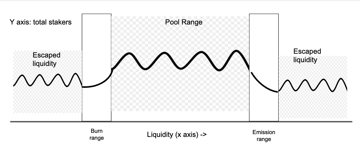
In my setup I define the particle inside of the box as the aggregate liquidity of the pool valued in an underlying asset. The goal is to incentivize users to remain within two points on the x axis, defined in ETH or USD, that form the boundaries of optimal liquidity levels. Inside the range the particle (all liquidity) has movement that is roughly sinusoidal, but this is not important to keep track of. What is important is when that liquidity approaches one of the boundaries. At the boundaries, which are not fixed values of x but have a width w between two points on the x-axis, the liquidity begins to to tunnel by becoming a eq 1.2. Exponential functions happen to be a nice way of modeling a declining rewards model. So, then eq. 1.2 can then be thought of as the emissions of new tokens, or, burn of existing tokens, and the wave functions on the outside of the barrier are the escaped liquidity. The purpose of the tunneling function is to mitigate the amount of escaped liquidity by creating burn defined by eq 1.2 when liquidity hits the inside edge of the lower boundary and creating emissions when liquidity hits the inside edge of the upper boundary. Inside the boundaries, any incentive scheme (or none) could be applied. The result is a setup by which users can be corralled into a specific range of liquidity with changes to token supply only occurring when necessary. If the aggregate value of liquidity moves beyond the entire width of the barrier then the system has broken and the protocol should reconsider the parameters being used.
Conclusion
The quantum mechanical principles are applied for two reasons: to create a theoretical model for understanding liquidity, which abstracts the behavior of fundamental particles, and to use already derived solutions of Schrodinger’s equations to obtain an exponential decay that nicely describes how emissions and burn ought to be leveraged such that users are economically incentivized to maintain a specific range of liquidity in the pool. Ranged liquidity is the desirable outcome for protocols at maturity. Growth in liquidity cannot continue forever, because 1) inflation cannot continue forever, 2) users will eventually be compelled to sell after earning enough return and 3) new protocols will inevitably siphon liquidity. Incentives becoming rangebound is the optimal way to retain a reasonable level of liquidity over a long term.